How to Delete Duplicates in Google Sheets

In this article, we will talk about the most simple and convenient way to remove repetitions in Google Sheets tables.

Content:
1. How to highlight duplicates in Google Sheet
2. Key moment
3. Possible alternative

Cells with repeated data are quite common when working with spreadsheets. Especially when it comes to a large table. Even one unwanted duplication can make it difficult to work, give incorrect results. In other words, spoil the nerves of the user. It still makes sense to look at a small table line by line. But for a document of several dozen lines, this approach makes no sense. We need to look for a different approach.

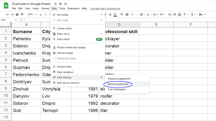
Google Sheets' arsenal of spreadsheet tools includes the removal of duplicates Data -> Data Cleanup -> Remove Duplicates.

The tool is handy and useful. However, in many situations, the user needs to do more than just “clean up” the table. But also to see which cells turned out to be duplicated. In other words, it would be good to just mark them for a start.

Further, the reader can get acquainted with one, the most universal technique for solving this problem.

The technique, which will be discussed, allows you to highlight the repeating cells with a color. A custom formula for the conditional formatting feature is used for this purpose.

For clarity, a very small table is taken. Let's try to find repetitions in it. First, select the columns in which you want to check the cells.

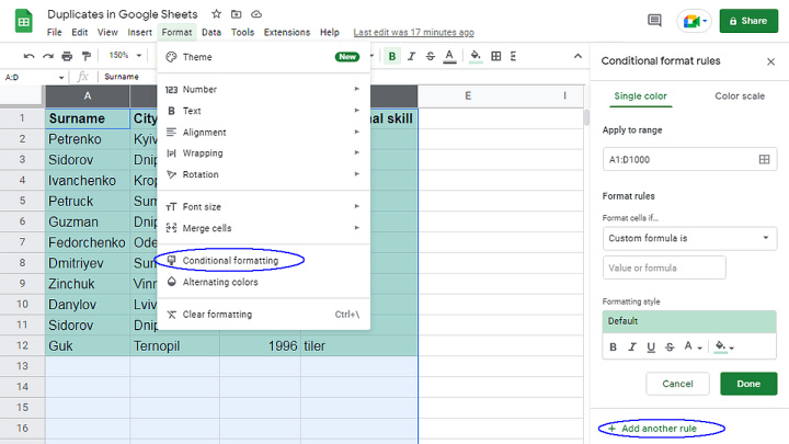
We go to the conditional formatting menu Format -> Conditional Formatting, where we find a window for setting formatting rules Conditional format rules.

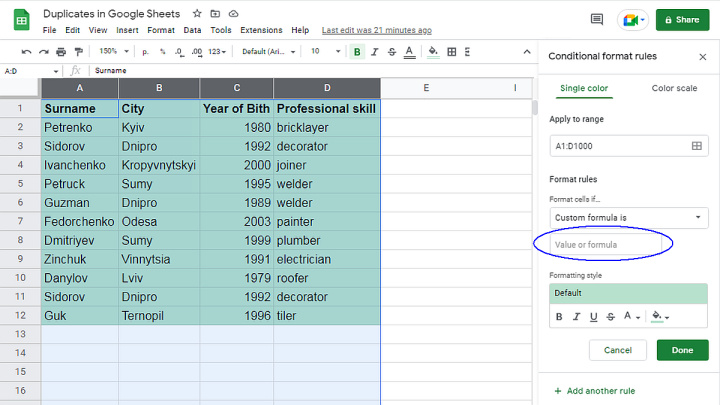
Please note that the field Apply to range is filled in automatically - the columns selected in the previous step are marked in it.

Go to the field Format cells if... The drop-down menu offers an impressive list of possible options. But you didn’t forget that we go our own way and create our own formula for finding duplicates? Therefore, without hesitation, click on the item located at the very bottom of the list Custom formula is...

We proceed to the most laborious stage of our work. Don't be afraid if everything doesn't work the first time.

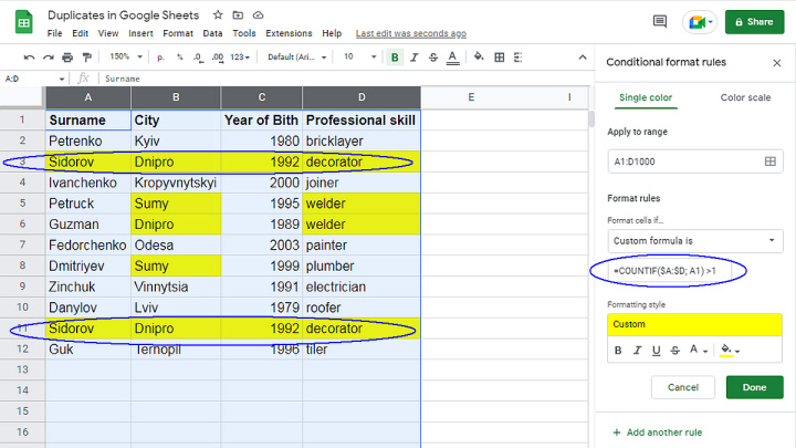
Now we enter the function =countif($X:$Y,A1)>1 into the field. X and Y denote the start and end columns of the range we need. In passing, I note that the function =countif is used if repetitions are searched for that correspond to ONE parameter. If there are SEVERAL parameters, then use another tool - the function =countifs.

Let's move on to how the detected repetitions will look like. This is done in the menu below the formula Formatting style. Everything is simple and clear here. You can choose between filling the cell with color or the characters within it.

Click Finish to complete the created formula and start working. Ideally, all cells with repeats will change color.

So, the function we created found all cells with duplicate data.

Here is an example of how the result can be used. Obviously, lines 3 and 11 are 100% repeated. It is possible that this is a table filling error. It is possible with a clear conscience to remove an extra line, or to merge identical lines.

If the reader does not like the technique described above, then we can offer one more trick. You can search for duplicates using the Remove Duplicates application from Ablebits. The free trial version is valid for 30 days. Remove Duplicates searches, marks, removes (merges) identical lines.

Apix-Drive is a simple and efficient system connector that will help you automate routine tasks and optimize business processes. You can save time and money, direct these resources to more important purposes. Test ApiX-Drive and make sure that this tool will relieve your employees and after 5 minutes of settings your business will start working faster.